What are VLMs?
Vision language models, or for short (VLMs), are multi-modal models that allow a (large) language model to understand images and perform tasks that have an image-based input. For example, asking the model how many dogs are in this picture and sending a picture along with the text to the model to be processed. When we add the capability of understanding other forms of input to a Large Language Model (LLM), we call them Large Multi-Modal Models (LMM).
How VLMs work?
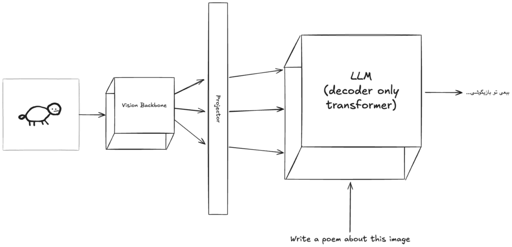
Visual language models usually consist of a vision encoder backbone model, a projection layer, and an LLM. The goal of the vision encoder is to compute a set of representative tokens from the input images and is usually trained on an image dataset separately.
The projector layer is supposed to take the computed tokens from the image backbone and project them to the LLM encoding space. In other words, it applies some transformations on image tokens to make them meaningful to the LLM.
The role of the LLM is pretty clear as well. It takes the projected image tokens as well as the raw text embedding and is supposed to generate relative results in return.
The process of feeding the image tokens to the LLM is also interesting. In most current works right now, the image tokens are fused with the text tokens at some intermediate layer inside the LLM, but there are some new models that take the image tokens or even raw images at the same time as the text, but they are still not performing well enough to completely replace the current methods of token fusion.
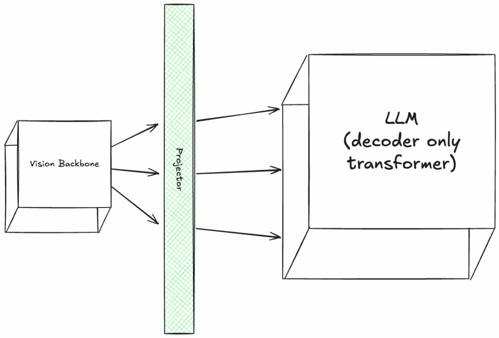
The training process of VLMs is also interesting. If we consider that we have a trained vision backbone and a trained LLM, the first step is to train the Projector layer to learn how to convert the image tokens to language tokens. BLIP-2 is the original paper that was published with this idea.
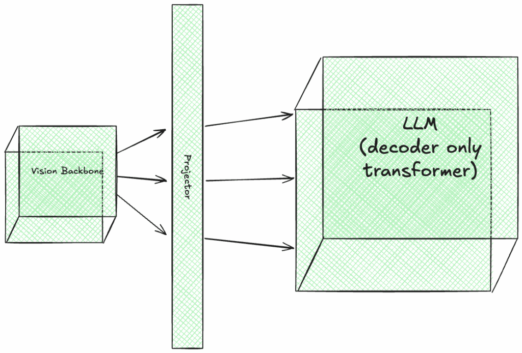
Then the next stage of the training includes fine-tuning all the modules, including the vision backbone and the LLM, on a visual instruction dataset. These datasets are similar to QA datasets, but with the additional image for each training record.
The following images are showing which modules are trained at each stage of training with green color:
Alright, now that we have a general understanding of what VLMs are and how they work, let’s see what the main problem that this paper is going to solve is.
The tradeoff of image resolution/accuracy-latency
It is shown in previous works that increasing the resolution of the input image has a direct positive effect on the performance of the model in terms of accuracy. But as always, there is a trade-off to consider here. When the image resolution is increased, the vision backbone models will probably need a longer time to compute the tokens for the image. The number of computed tokens will increase, and as a result, the LLM will require a longer time to process all the input tokens to generate the output. The time that it takes for a Feed-Forward flow to complete in deep learning models is called the pre-filling time, and the time it takes for the LLM to generate the first output token is considered an efficiency metric called Time to first token or TTFT in short. It is obvious that if we have a VLM that takes a longer time to process the input image and generates more image tokens, that in turn will cause an increase in the pre-filling time of the LLM, it will have a longer TTFT, which is not a good thing in general.
By combining the TTFT metric with the accuracy, we can plot a curve that can depict the tradeoff that happens between accuracy and TTFT when the input image resolution increases. This is called a Pareto-optimal curve.
So, is there a way to improve the accuracy of the model by using high-resolution images while keeping the TTFT metric relatively low?
Well, according to what we said, there are 3 main reasons that the TTFT increases:
- The vision backbone requires a longer time to compute the tokens
- The vision backbone generates more tokens when the image resolution increases which increases the pre-filling time of the LLM
- The time that it takes for the LLM to take the input and generate the first output token.
In this work, Apple researchers are trying to move towards a better solution by tackling the first 2 reasons and introducing an improved vision encoder as the backbone that is both faster than the existing image encoders and generates fewer tokens per image.
Swapping the image encoder of the VLM
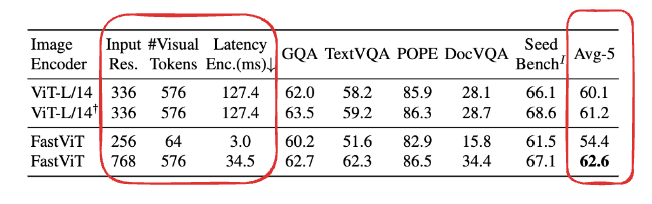
This paper is actually continuing the work that the same team of researchers conducted in the FastViT paper, which is a brand-new architecture for image encoding. We’ll look at the main architecture and innovations of FastViT here as well, but the first thing that the authors try here is to place FastViT, which is a hybrid convolutional-transformer-based architecture that is already faster than the family of vision transformers, and as it is reported and you can see in the results table shown below, FastViT is much faster and creates fewer tokens for the input images with the same image resolution. It does, however, show a lower average accuracy score for the same input image resolution, but with an increase in the image resolution, we can see that FastViT is still much faster (about 4 times) and achieves a better average accuracy.
Now that we saw FastViT is a faster image backbone that can achieve the same accuracy in VLMs as the existing image backbone models, let’s take a look at its architecture and what makes it a good and efficient image backbone.
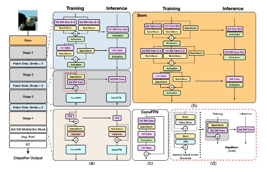
The main layers are abstracted and are shown on the left side of this image taken from the original paper. Then, each layer is shown in more detail on the right side of the image with the same corresponding colors.
The first layer called the stem is our input layer that receives the original image and extracts low-level details (ex. the edges and lines, etc.) from the image and performs downsampling to reduce its dimensions and passes the feature maps to the next layer where the generated tokens are mixed using a brand-new module called RepMixer that is influenced by ConvMixer and is further processed in another convolutional feed-forward network to extract higher-level features.
The third layer is called Patch Embedding and it was introduced to image processing through vision transformer architectures where the input image is broken into patches and each patch is then projected into a vector that would act as the token for that part of the image. In convolutional patch embedding, we’re still breaking the image into patches, but use separate depth-wise convolutions for processing each patch which acts as a projection layer, but requires fewer parameters and retains the spatial information present in the image. We’re also downsampling the feature maps in this layer as well to only pass high-level information to the next layers and reduce the computations.
The stack of feature extraction from layer 2 and patch embedding can be repeated multiple times and is repeated 3 times here, before moving to the last feature extraction layer which is similar to what we have in layer 2, but with the addition of using a self-attention module instead of RepMixer for mixing the computed tokens.
The final layers are the standard layers you can find in any image classification model that flatten the computed feature maps and apply a fully connected MLP to classify the object in the image.
Now let’s review some important decisions that make this model more mobile-friendly and efficient:
Wide use of Depth-wise Convolutions
This isn’t the right place to go into the details of how convolutions work, but you can think of it as a limited receptive field that is used to process a part of an image. (Think: seeing a room in the dark with a flashlight that only lights up a single part at a time.)
Normal convolution layers look like this:
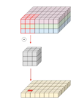
At the top we have an input image with 3 channels (like RGB), and we’re applying a convolution kernel of size 3×3 to create a feature map. As you can see, this normal convolution is converting 9 pixels into 1 pixel in the next feature map. This means if we want to have 20 feature maps for the next level in the network, we need to apply 20 separate kernels and stack the output feature maps to reach the desired output channel. The total number of parameters that this adds to our model can be computed as input-ch * output-ch * kernel-width * kernel-height. In this example, the number of parameters would amount to 540 parameters (the numbers will scale very fast in deep nets).
Depthwise convolutions and Depthwise separable convolutions are attempts at making the convolution operation more efficient and they are widely used in the family of MobileNet and EfficientNet models.
Let’s take a look at what Depthwise separable convolution looks like:
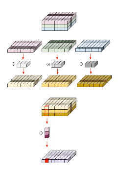
As you can see, the trick is to apply a separate kernel with a channel size of 1 to each channel in the feature map to produce the next feature map, and then to collapse the intermediate feature maps computed from each channel and effectively get the same result as we would from the normal convolution, we apply a point-wise convolution to convert them to a single channel. The total number of parameters for depth separable convolutions are computed as: depthwise params + pointwise params = k * k * input-ch + 1 * 1 * input-ch * output-ch. so in a similar setup as above, we’d have: 27 + 30 = 57 learnable parameters.
Convolutional token mixer for early stages
One of the important contributions of the FastViT paper is introducing RepMixer for token mixing, which is a convolutional token mixer that requires a lot fewer parameters when compared to self-attention and is more efficient than ConvMixer due to re-parameterization at inference time.
Let’s talk a little bit about token mixing and what it means:
As you know our input image is broken up into separate parts during processing and we’re calling them a Patch, each patch is computed separately from a grid in the image and only includes the information about that part of the image, like a single puzzle piece, in token mixing, the main goal is to add more global context information from the other puzzle pieces to each patch.
In FastViT, a convolutional token mixer is used in the early stages due to computational efficiency, followed by a single self-attention token mixer in the last stage.
Training time over-parameterization and re-parameterizing at inference
As mentioned earlier, FastViT is heavily using DepthWise convolutions that have fewer parameters when compared to standard convolution operations. Having fewer parameters is good if we can reach the same accuracy/performance, but on paper, it generally means a model with fewer parameters has less capacity to learn. To overcome this potential limitation, a technique is used called training over-parameterization where the number of parameters is more than the parameters that are used during inference. This is depicted in the FastViT visual architecture as well.
Making some improvements to the FastViT model
Let’s get back to the main goal of this paper: Improving the Pareto-Optimal curve for Accuracy Vs TTFT in VLMs.
We saw that by using FastViT as the image encoder in VLMs, we get an instant boost in the latency and can even match the accuracy of the leading models while being more efficient.
By applying some minor changes to the FastViT model, the authors are introducing a new model called FastViTHD, that has the following architecture:
Let’s go over the changes in this architecture compared to the original FastViT:
Using 2 self-attention token mixing stages
There are 2 main reasons for adding an extra stage with self-attention to the architecture: Increasing the scale of the image encoder has a direct impact on improving the generalizability of the model; self-attention blocks are able to generate better enriched tokens by using all the available tokens and performing pairwise dot products to generate the next tokens.
But there is the problem with having more parameters that makes it sub-optimal to just add a new self-attention layer to the model; that’s why this issue is mitigated by adding another layer of downsampling to the architecture:
Downsampling by a factor of 32 instead of 16
Adding a new layer of downsampling to the architecture means that the final self-attention layer needs to perform fewer computations, and since we have a smaller feature map by the last downsampling, we’re going to have fewer tokens by the end, that are likely to include the same amount of information as before because of having another layer of self-attention.
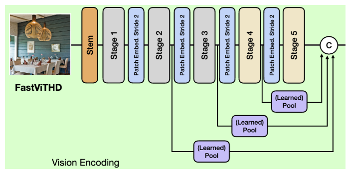
Multi-Scale Features
Another change in the architecture is using the features from different layers and different scales as the output of the Vision Encoders instead of just picking the features from the penultimate layer.
Features at different levels have different granularity and usually include complementary information that, when aggregated, can lead to a better overall performance.
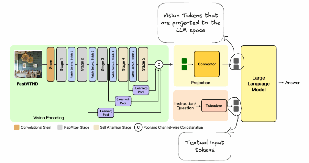
At last let’s take a look at the final architecture of FastVLM with FastViTHD as the main vision encoder:
Conclusion
We looked at the main parts of a new vision encoder that was introduced by Apple that tries to improve the Pareto-optimal curve of accuracy over time to the first token in vision language models, and as you can see in the presented results, when combined with the Qwen LLM family, FastViTHD has a much lower TTFT while being able to show good performance as well.
